I’ve been postponing the post for this fun small project for many weeks. Don’t blame me, I’ve still been working on more project euler problems and studying for the AWS Data Engineer Certification.
Anyway, it’s better late than never.
Just to give a small introduction about what this post is about: I’ve seen that it is possible to use NetworkX python library to get the graph representation of a real map using OpenStreetMaps, it’s not only a graph connection with nodes and edges, it also includes some road metadata that could be used as a weight for edges, at this point, you probably know where I’m pointing to.
So, think a bit about maps, what can you do with them?
- Find if there is a path between two positions
AandB. - If there is a path between
AandB, which one is the shortest? - If there is a path between
AandB, which one is the fastest?
and there are a lot of more questions that you can have and can be answered with a map, some easier than others.
However, at this point let’s focus only on the third one, which in some sense also involves the number 1 and 2.
So, the obvious question here is, how?. Unless, you’ve never taken a class on algorithms, you already know the famous Dijkstra algorithm, which is used to find the shortest path in a graph with some limitations.
I’m not going to explain how Dijkstra’s algorithm works because it’s really easy to find info about it on internet, instead I’m going to focus on how to build the application.
Getting the position
At the beginning, I deployed this project using latitude and longitude, however it’s really impractical as it’s easier for humans to know the street name instead of those pairs of values.
First step is to translate street or locations to latitude, langitude values. It could be a difficult task because it implies NLP algorithms, however OpenStreetMap allows us to use its API to find it without further troubles.
def get_lat_lon(address: str) -> Optional[Coordinates]:
    url = "https://nominatim.openstreetmap.org/search"
    params: Dict[str, str | int] = {"q": address, "format": "json", "limit": 1}
    response = requests.get(url, params=params, headers=HEADERS)
    if response.status_code == 200 and response.json():
        location = response.json()[0]
        return Coordinates(
            latitude=float(location["lat"]), longitude=float(location["lon"])
        )
    return None
Validating positions
The biggest issue for this application is downloading and plotting the maps, the problem is that if you want to find the shortest path between Paris and Berlin, then you have to download a map containing both and that is really big/heavy. So, for now we will also limit it to locations in the same city.
If we know the latitude and longitude for the source and destination, then we have to check if both are in the same country and city:
def get_current_location(
    coordinates: Coordinates,
) -> Tuple[Optional[str], Optional[str]]:
    latitude, longitude = (
        round(coordinates.latitude, 6),
        round(coordinates.longitude, 6),
    )
    url = f"https://nominatim.openstreetmap.org/reverse?format=json&lat={latitude}&lon={longitude}"
    response = requests.get(url, headers=HEADERS)
    data: Dict[str, Dict[str, str]] = response.json()
    if "address" not in data:
        return (None, None)
    address = data["address"]
    city: Optional[str] = address.get("city", None)
    country: Optional[str] = address.get("country", None)
    return (city, country)
Getting node id
So far, we still work with positions and latitude and longitude, however in graphs, we prefer to work with nodes and edges. Think for a moment, do we really need to know what is the latitude and longitude of each position? Isn’t it enough to have nodes represented by some id and edges connecting those nodes and having some length?
We don’t have to worry about geographic positions, but can abstract themo to an id. NetworkX allows us to download a graph knowing the city and country, which we already have from the previous step. This graph has nodes and edges, so our task is to map the position for source and destination to a valid id in the graph.
def get_node_id(graph: Union[MultiDiGraph, NGraph], location: Coordinates) -> NodeId:
    return cast(NodeId, ox.nearest_nodes(graph, location.longitude, location.latitude))

G = download_graph(country, city)
graph: Graph = generate_graph(G)
source = get_node_id(G, source_coordinates)
destination = get_node_id(G, destination_coordinates)
there are faster ways to calculate it, like caching the map and storing some data for the map in dynamo, but it will be explained later.
Graph algorithms
This is by far the most interesting section, here we don’t have to think in maps, instead in the abstract representation: graph.
If you remember the introduction, our goal is to find the fastest path, not the shortest path, both terms can be misunderstood as they are commonly attributed to the same thing, but in the fastest path we want to minimize the time, and in the shortest path the goal is to minimize the length.
Of course, both quantities are related, if you remember your physics classes or follow your intuition you can get:
\begin{aligned} \Delta t = \frac{\Delta \mathrm{length}}{\mathrm{speed}} \end{aligned}
However, this is only true if the speed is constant and equal on all edges, which of course is something we can’t guarantee, there are some roads with speed limit and then we have a constraint for each edge, to refine this idea, consider a discrete approach:
\begin{aligned} \Delta t = \sum_{i} \frac{\Delta \text{lengt}h_{i}}{\text{speed}_{i}} \end{aligned}
where length[i] is the length of edge[i] and speed[i] its maximum allowed speed.
It’s the only modification we have to do, and the data for the maximum allowed speed is provided by OpenStreetMaps.
If you remember correctly, Dijkstra is an algorithm to find the shortest path between a source to all the other nodes in the graph, which is not the case for the application, it will work, but there are better ways.
A* algorithm
A* is a heuristic algorithm, which uses the fact that given two nodes, if we can approximate and find a lower bound for the distance between them, then it’s possible to have a better idea about which is the next best node, this will reduce the number of iterations drastically.
If you remember well, each node represents a position on a real map, this means that it has a latitude and longitude, then the eulerian distance between these two nodes is:
\begin{aligned} d = \sqrt{(\Delta x)^2 + (\Delta y)^2} \end{aligned}
wait, the earth is not flat!, it means the minimum distance between two positions in the earth surface is not a straight line, that’s also the reason why we are using latitude and longitude instead of x, y, z positions. Instead of using eulerian distance, we have to use Haversine distance:
\begin{aligned} d = 2r\arcsin\bigg( \sqrt{\frac{1-\cos(\Delta \phi) + \cos\phi_{1}\cdot \cos\phi_{2}\cdot (1-\cos(\Delta \lambda))}{2}} \bigg) \end{aligned}
and $r \approx 6371 \text{km}$.
This is my implementation in Rust, don’t ask me why I wrote it in rust, I just wanted to try something new.
let destination_node = graph.nodes.get(&destination).unwrap().clone();
while let Some(State { weight: _, node_id }) = priority_queue.pop() {
let weight_to_node = weight_from_source
.get(&node_id)
.copied()
.unwrap_or(INFINITY);
if node_id == destination {
return Some((
previous_node,
visited_edges,
Vec::from_iter(active_edges),
weight_to_node,
iteration,
));
}
let current_node: Node = graph.nodes.get(&node_id).unwrap().clone();
if visited_nodes.contains(&node_id) {
continue;
}
visited_nodes.insert(node_id);
let next_nodes_id: Vec<NodeId> = current_node.next_nodes;
for next_node_id in &next_nodes_id {
iteration += 1;
let next_node: Node = graph.nodes.get(&next_node_id).unwrap().clone();
let current_edge_id: EdgeId = (node_id, *next_node_id);
let current_edge: Edge = graph.edges.get(¤t_edge_id).unwrap().clone();
visited_edges.push(current_edge_id);
active_edges.remove(¤t_edge_id);
let edge_weight: f64 = (current_edge.length / 1000.) / (current_edge.maxspeed as f64);
let destination_distance: f64 = find_distance_by_nodes(
next_node.lat,
next_node.lon,
destination_node.lat,
destination_node.lon,
)
.await;
let heuristic_weight: f64 = destination_distance / max_speed_allowed;
let new_weight: f64 = weight_to_node + edge_weight;
if weight_from_source
.get(next_node_id)
.copied()
.unwrap_or(INFINITY)
> new_weight
{
weight_from_source.insert(*next_node_id, new_weight);
previous_node.insert(*next_node_id, node_id);
priority_queue.push(State {
weight: new_weight + heuristic_weight,
node_id: *next_node_id,
});
let nodes_to_visit: Vec<NodeId> =
graph.nodes.get(&next_node_id).unwrap().clone().next_nodes;
for to_visit_node_id in &nodes_to_visit {
active_edges.insert((*next_node_id, *to_visit_node_id));
}
}
}
}
A* enhanced algorithm
This is my modification of the A* algorithm, it can’t guarantee you a path but in most of the cases I’ve tested, it was able to beat A* and find the same solution in fewer iterations.
My idea is to use a level max distance that is constantly updated for a node $u$. If the haversine distance is greater than 2 * best distance / ln(1 + best distance) then the node is skipped, the best distance is calculated as the minimum between the Haversine(source, destination) and Haversine(u, destination)
if level_max_distance != INFINITY {
    level_max_distance = f64::max(level_max_distance, destination_distance);
} else {
    level_max_distance = destination_distance;
}
if best_node_distance != INFINITY {
    if destination_distance * f64::min(1.0, (1.0 + best_node_distance).ln())
        > 2.0 * best_node_distance
    {
        continue;
    } else {
        best_node_distance =
            f64::min(source_to_destination_min_distance, destination_distance);
    }
}
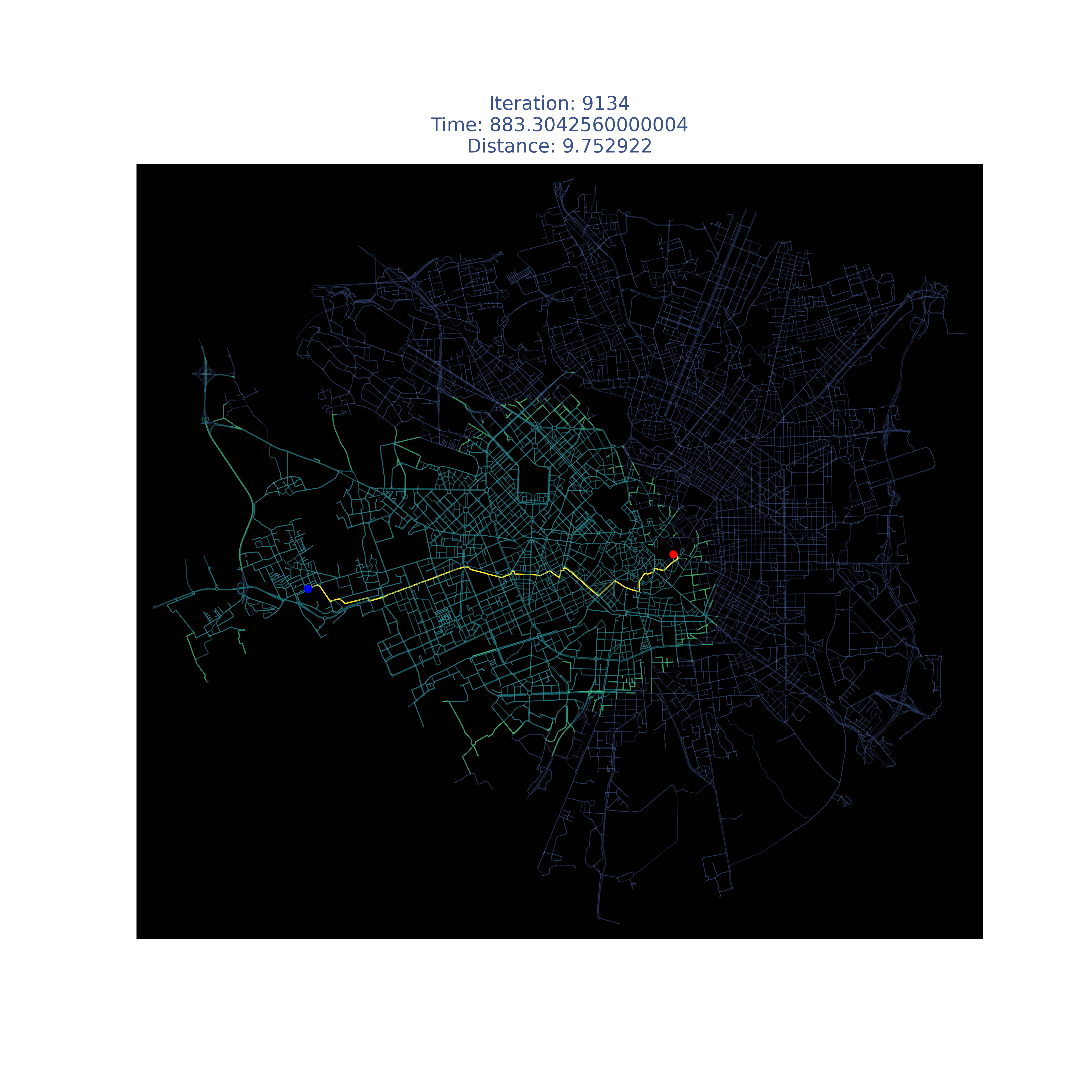
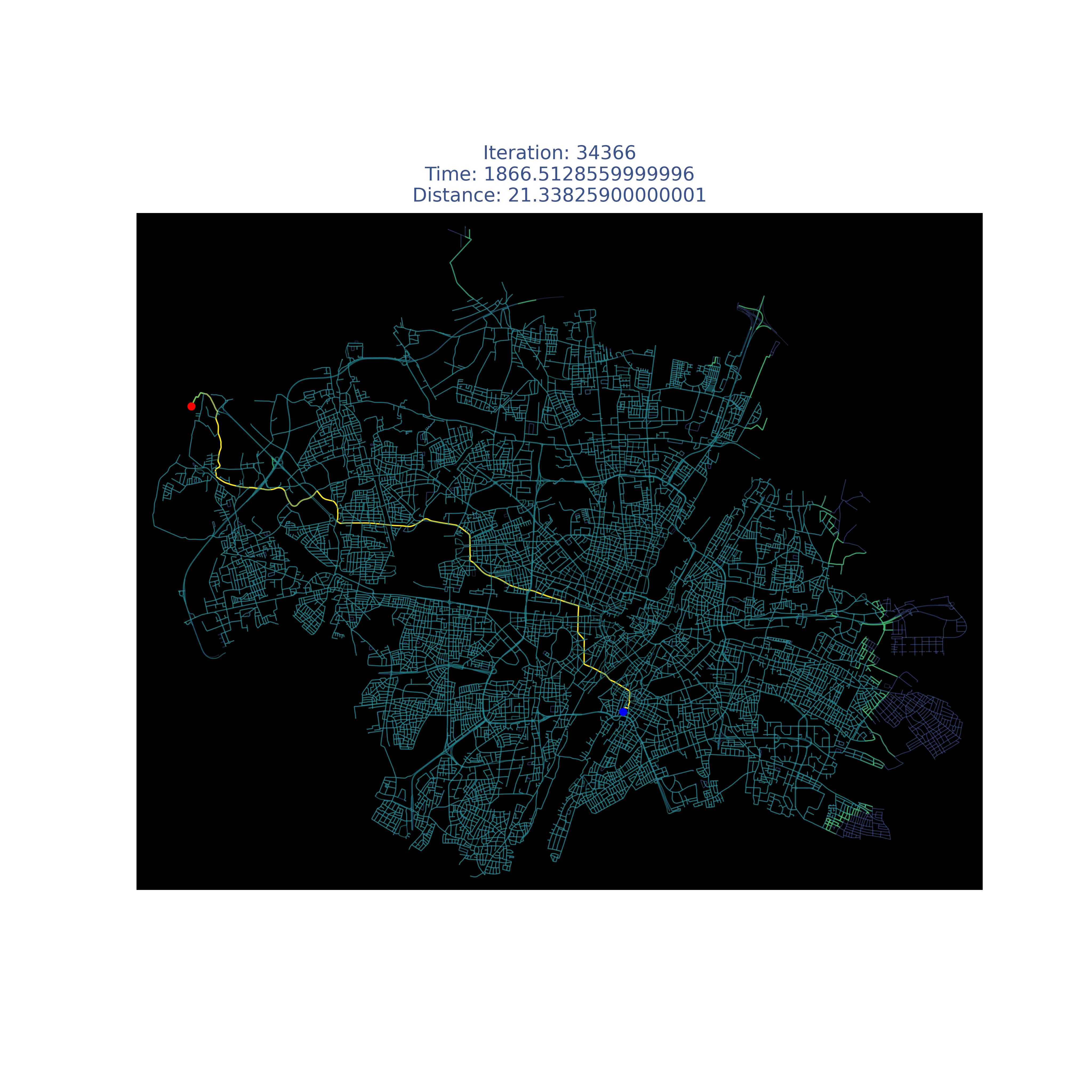
It means that nodes that make a step backwards are penalized more than nodes that make you move forward to the destination. It will be clearer when you can see the plots.
Plotting
NetworkX already allows us to plot a downloaded map and customize nodes and edges, so the remaining step is to find the visited edges and the edges that belong to the fastest path.
def save_graph(
    graph: MultiDiGraph,
    edges_in_path: Set[EdgeId],
    visited: Set[EdgeId],
    active: Set[EdgeId],
    source: NodeId,
    destination: NodeId,
    solution_key: str,
    dist: float,
    time: str,
) -> str:
    node_size: List[float] = []
    node_alpha: List[float] = []
    node_color: List[Color] = []
    for node in cast(List[NodeId], graph.nodes):
        if node in (source, destination):
            node_size.append(POINT_SIZE)
            node_alpha.append(POINT_ALPHA)
            if node == source:
                node_color.append("blue")
            else:
                node_color.append("red")
        else:
            node_size.append(NODE_SIZE)
            node_alpha.append(NODE_ALPHA)
            node_color.append("white")
    edge_alpha: List[float] = []
    edge_color: List[str | Tuple[float, float, float, float]] = []
    edge_linewidth: List[float] = []
    for edge in graph.edges:
        edge_id = (edge[0], edge[1])
        if edge_id in edges_in_path:
            edge_color.append(PathEdge.color)
            edge_alpha.append(PathEdge.alpha)
            edge_linewidth.append(PathEdge.linewidth)
        elif edge_id in visited:
            edge_color.append(VisitedEdge.color)
            edge_alpha.append(VisitedEdge.alpha)
            edge_linewidth.append(VisitedEdge.linewidth)
        elif edge_id in active:
            edge_color.append(ActiveEdge.color)
            edge_alpha.append(ActiveEdge.alpha)
            edge_linewidth.append(ActiveEdge.linewidth)
        else:
            edge_color.append(UnvisitedEdge.color)
            edge_alpha.append(UnvisitedEdge.alpha)
            edge_linewidth.append(UnvisitedEdge.linewidth)

    fig, ax = ox.plot_graph(
        graph,
        node_size=node_size,  # type: ignore
        node_alpha=node_alpha,  # type: ignore
        edge_color=edge_color,  # type: ignore
        edge_alpha=edge_alpha,
        edge_linewidth=edge_linewidth,  # type: ignore
        node_color=node_color,  # type: ignore
        bgcolor="#000000",
        show=False,
        close=False,
    )
    title: str = "\n".join([f"Distance: {dist} km", f"Time: {time}"])
    ax.set_title(title, color="#3b528b", fontsize=10)
Final considerations
I’ve explained in general terms how this project was built, however there are many more details that I couldn’t explain, nevertheless I want to make a quick mention to them.
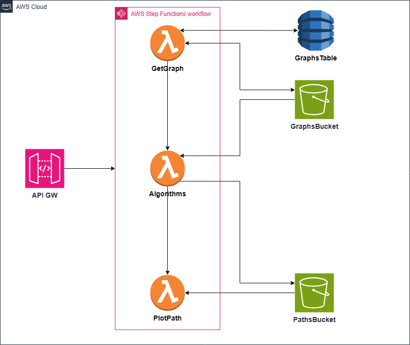
- Step functions to orchestrate the lambda functions.
- Preload most common graphs and upload them to S3 with a unique graph id and store it in dynamo for quick queries.
- If the map is already in S3, then no need to download the complete graph, only a small radius around the position to calculate the node id.
- Instead of using the heavy map from
NetworkX, use a simplified graph containing only the necessary information. Store it in S3 as well. - Deploy an API GW and a presigned url to retrieve the plot.
- Use lifecycle configuration to delete old plots.
Results
| Place | Dijkstra | A* |
|---|---|---|
| Milan | 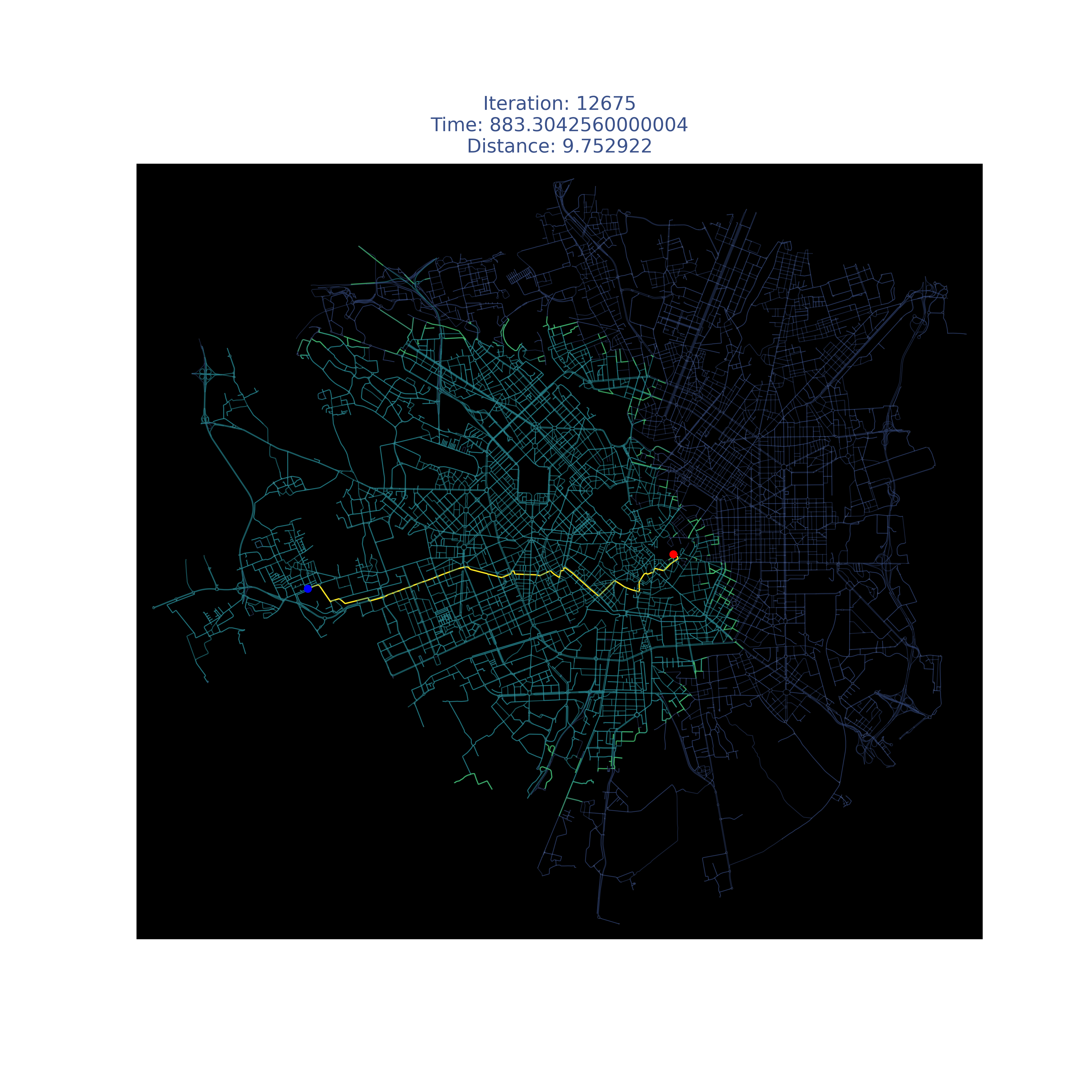 |
 |
| Munich |  |
 |
| Paris | 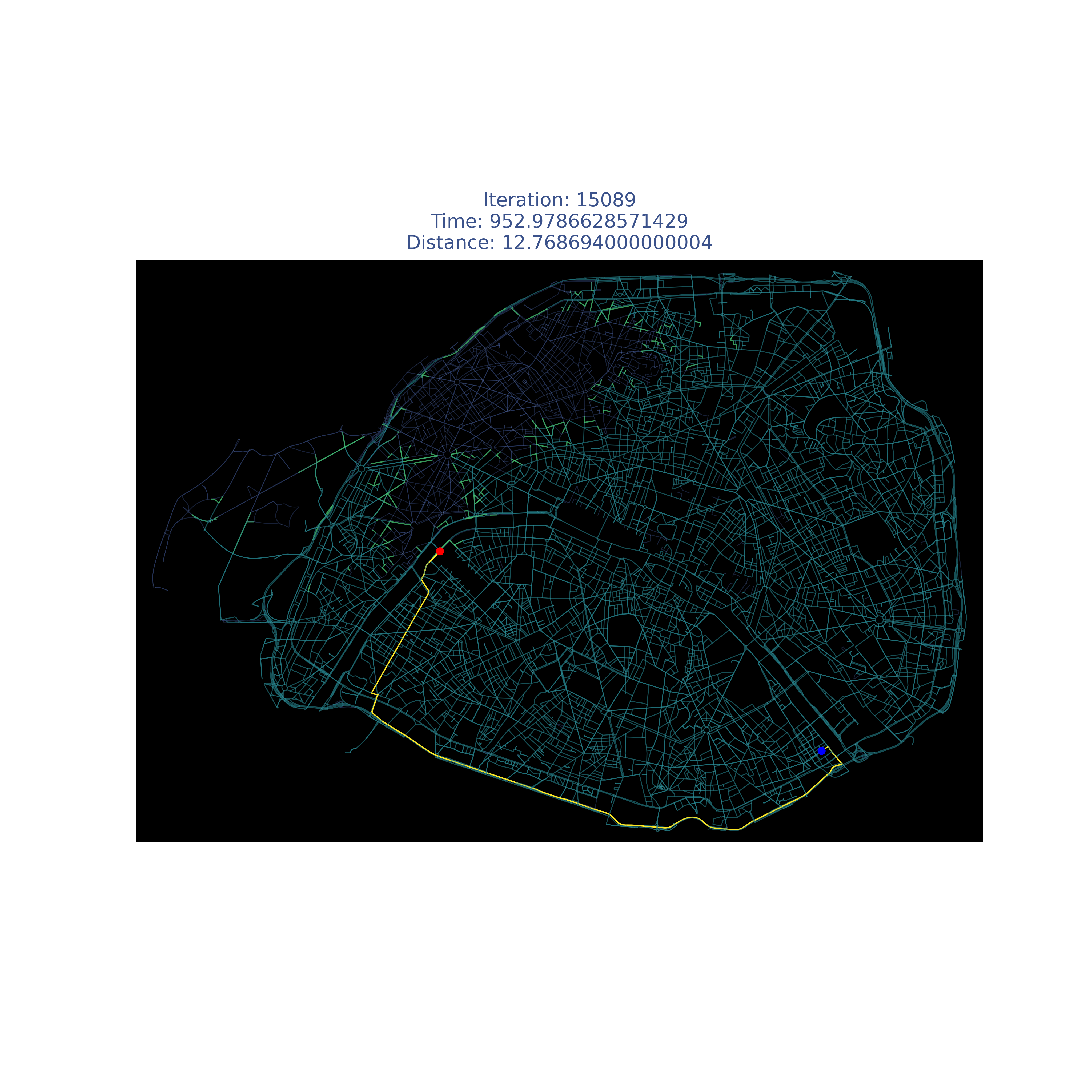 |
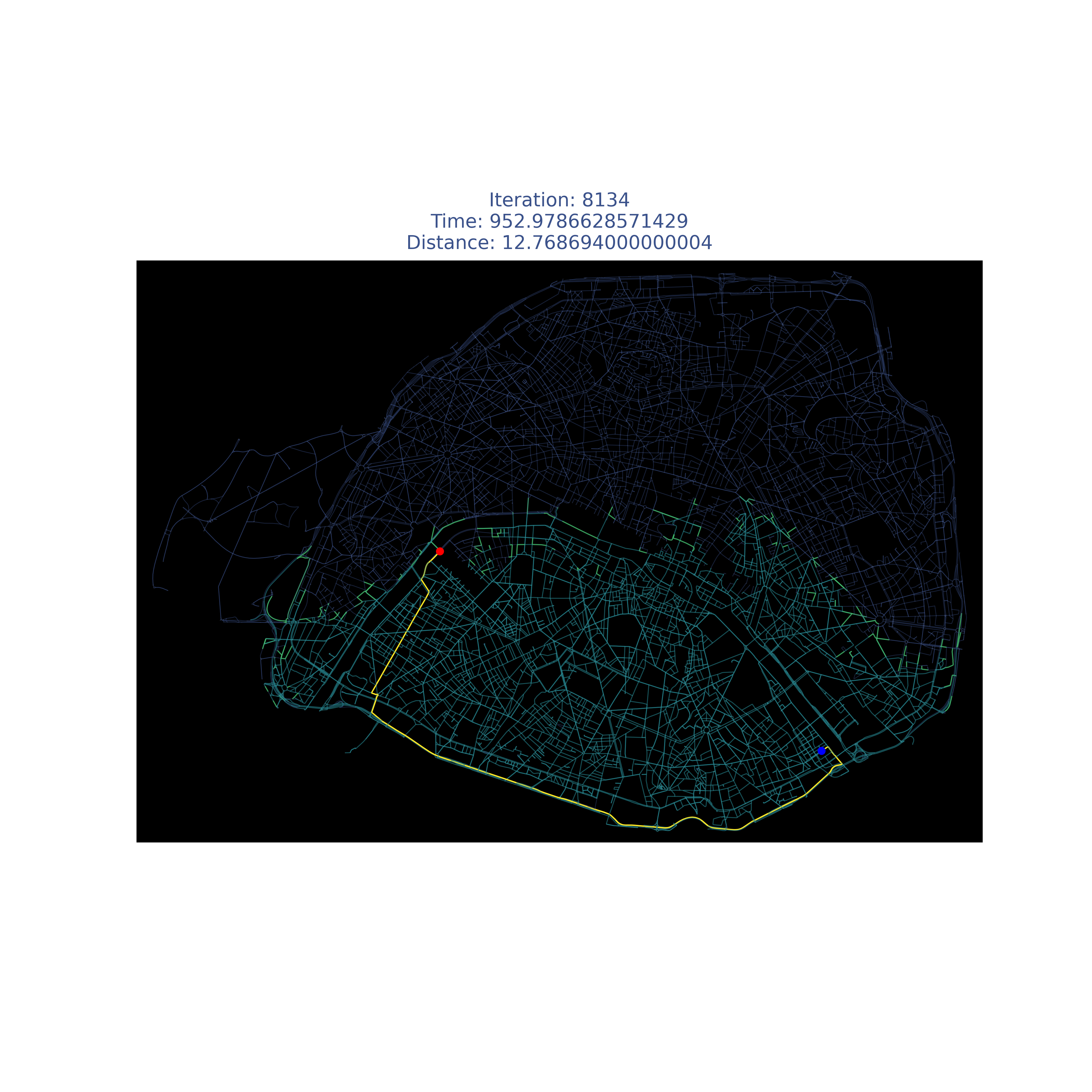 |
Compare it with my modified version :)
| Place | A* enhanced |
|---|---|
| Milan |  |
| Munich |  |
| Paris |  |
You can try it running:
curl -i "https://u4buvcwtvp4miopkjjqadffazq0zjric.lambda-url.us-east-1.on.aws/?source=Paris,%20Gros-Caillou&dest=Paris,%20Charonne&algorithm=a_star_enhanced"
It could takes a few seconds or minutes depending how big is the map and if the lambda is already warm.
Further work
I still have some optimizations pending that could make this project more interesting. One of the biggest limitations is that plotting/downloading the graph can take long time, for example for Lima, Peru is almost impossible to plot in the lambda because it has many roads and the map is 4 times bigger than others. It’s not an issue with the algorithm because Rust runs very fast and can find the path in few seconds, the issue is in how NetworkX is plotting the map, so it involves making some changes in the library or building my own library to plot it, however I think it’s really out of scope for now.
Next big improvement I’d like to add is to be able to find the path for different cities or different countries, as I mention at the beginning, the problem is that the map could be very large and then almost impossible to get all data in a reasonable time, but then the question is how google maps can do it? The answer is based on the fact that each city could be considered as a small isolated graph. This works because there are only a few roads that can be used to go from city A to city B, so it is enough to find the best solution in each isolated graph, and then include some more edges only at the border that are used as the main roads to move between cities. There is a clever way to compress this idea and it’s with graph layers, if you zoom-out in google maps, you can stop seeing some roads, you may think it’s because of a UI decision to keep it minimalistic and not oversaturate the map, but actually it’s a really good explanation about how the layers works because in large distances, we only care about finding the optimal path between these main roads (upper layers) and not in the smaller ones (lower layer). Of course, it’s not as easy as I describe it here, google also implements some graph simplifications like removing some edges that could be considered subotpimal or not necessary when we are working in an upper layer.
Additionally to that, we can even simplify more the graph abstraction. If we run Floyd Warshall for a city, we can make a statistic to know which roads are used the most and which are never used, then we can give a priority to these edges or delete some of them because we have this pre-computed information before, leading to fewer iterations.
Lastly, if we want to implement the fastest path in real time, we should get traffic information in real time to have a better estimate of the time it could takes to traverse a road. I don’t know at the moment if there is any algorithm that works with approximate/dynamic graphs, but it’s of course an interesting problem. However, since the code in Rust can run in a few seconds, we can simply consider a static graph every time there is a query with new traffic information, so we don’t have to deal with dynamic updates.